Microarray Data processing with RMA
Overview
Teaching: 20 min
Exercises: 20 minLearning Objectives
Understand and explain Background correct, normalise and summarisation steps for microarray data
The processes of RMA
The RMA algorithm performs steps of data processing discussed in class.
- Background correction.
- Normalisation.
- Summarisation (calculating feature-level data)
These steps are performed in order, and yield a processed data set size that is considerably smallar than the data set prior to processing. While the starting object is an AffyBatch object, the result is an ExpressionSet. `
Plotting the signal densities from raw CEL files
The hist() functions from the oligo package show the signal densities of data from each sample in overlaid line plots.
hist(gse33146_celdata,
     main='CEL file densities before normalisation or background correction',
     lwd=2)
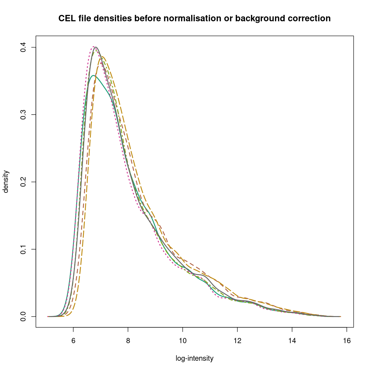
plot of chunk affy-densities
As you can see, each sample does look like it comes from a similar kind of distribution for all six CEL files, but the exact distributions clearly differ. The prcessing steps of RMA address these issues to provide estimates for each feaature (transcript).
The need for background correction
Microarray data contains ubiquitous background noise, so an important first task is removal of background noise. Different algorithms deal with background differently. Most Affymetrix expression microarrays are designed with probe pairs, where one probe is a perfect match (PM) to the target and one is a single base mismatch (MM) to the target. Methods like Affymetrix’s own MAS5 algorithm use the difference between PM and MM hybridisation to addreess background noise. The RMA algorithm ignores the MM probes, and so must address background correction directly as a property of hybridisation.
The RMA model is to model the perfect match (PM) signal as a sum of the real signal for probe \(j\), from probeset \(k\), on array \(i\).
\[\text{PM}_{ijk} = \text{bg}_{ijk} + s_{ijk}\]The key part of the model is to assume that the true signal is drawn from an exponential distribution
\[s_{ijk} \sim \text{Exp}(\lambda_{ijk})\]while the background component (both optical noise and non-specific hybridisation) is drawn from a normal distribution that depends only on the array:
\[\text{bg}_{ijk} \sim \mathcal{N}(\beta_i,\sigma^2_i)\]The background removal step of RMA estimates and removes this second component.
The gcrma algorithm differs from rma in assuming the background also depends on the GC content of the probes.
raw_nobg <- backgroundCorrect(gse33146_celdata)
Background correcting... OK
hist(raw_nobg,xlab='log intensity',
     main="CEL file densities after RMA background correction",
     lwd=2,which='pm')
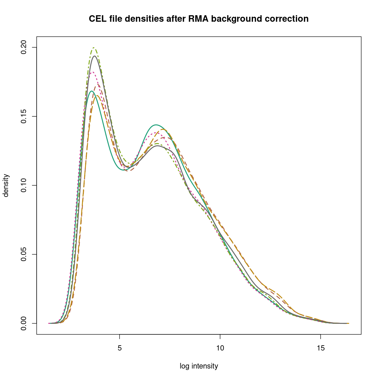
plot of chunk bgcorrection
The need for normalisation
Sample normalisation in RMA is performed via quantile normalisation of the probe level data, as discussed in class. This allows samples to be compared to each other assuming the data arise from thesame parent distribution.
Quantile normalisation puts the data on a common empirical distribution.
oligo_normalised <- normalize(raw_nobg,method='quantile',which='pm')
Normalizing... OK
hist(oligo_normalised,lwd=2,xlab='log intensity', which='pm',
     main="CEL file densities after quantile normalisation")
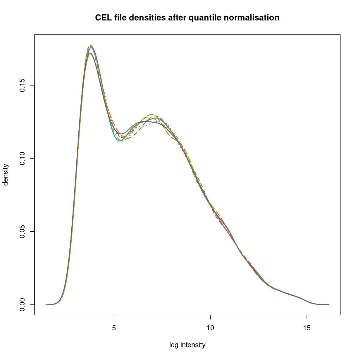
plot of chunk oligo_normalization
Summarisation: from probe-level to feature-level data.
oligo_summarised <- rma(oligo_normalised,background=FALSE,normalize=FALSE)
Calculating Expression
hist(oligo_summarised)
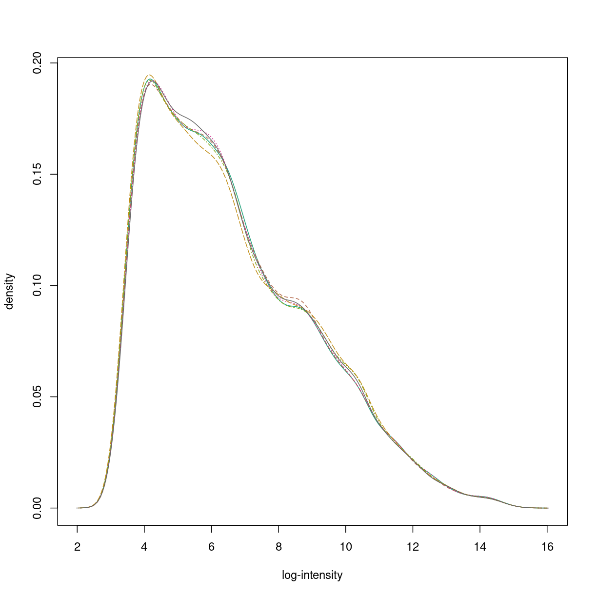
plot of chunk oligo_summarised
The summarisation step reduces the size of the data for each sample to the number of measured transcripts (or genes, or exons, depending on the array). These are referred to as “features”, or “probesets”, and the resulting ExpressionSet is “feature-level” data. The summarisation step in rma is performed for each probe-set over all background-corrected, quantile-normalised samples using the median polish algorithm.
Performing RMA in R
Performing RMA in R is relatively straightforward. The function, rma() from the affy package takes in an AffyBatch object. The function basicRMA() from the oligo package takes in an ExpressionFeatureSet object. Hence, the following one line of
code performs RMA normalisation, and returns an ExpressionSet object containing the
background corrected, normalised, and summarised expression data.
gse33146_eset <- rma(gse33146_celdata)
Background correcting
Normalizing
Calculating Expression
gse66417_eset <- rma(gse66417_celdata)
Background correcting
Normalizing
Calculating Expression
Try it
If you get help on
rma()using eitherhelp(rma)or?rma, you can see how to run the same process without background correction or normalisation. Try it!
Manipulating an ExpressionSet object
Earlier, we have alluded to the data contained in an ExpressionSet object. We can access each of these pieces of data using the following functions:
| Data | Type of information | Function |
|---|---|---|
| Annotation | Chip information | annotation() |
| PhenoData | Phenotype data | pData() |
| Expression | Normalised gene expression | exprs() |
| Experiment data | Experimental information | experimentData() |
| Feature data | Probeset data | featureData() |
The phenotype data for each of the samples are retained after rma, so you should be able to see that information
You can also try, running RMA without background correction, or without quantile normalisation, and plot the densities.
Key Points
RMA, the most widely used processing algorithm for Affymetrix data, is implemented in R using the
rma()function in theoligooraffypackages, depending on how the data was imported.The steps of background correction, quantile normalisation, and summarisation are performed in order to obtain feature-level data