Overview

Teaching: 15 min
Exercises: 0 min

Learning Objectives

• Introduction to Sleuth

What is Sleuth?

Sleuth is used for differential analysis of gene expression data. Sleuth will be run using R. The program makes use of Kallisto quantification and bootstrapping to improve statistical analysis. Sleuth overcomes problems previously faced in separating biological variance from inferential variance. This leads to improved False Discovery Rates (FDR) in identifying the differentially expressed.

Getting Started with Sleuth

The files used here can be downloaded as described in Setup, as well as how sleuth was set up.

If continuing with outputs from kallisto, move the output folders into ~/Desktop/RNA-seq/Sleuth_files.

The following commands are completed using Rstudio. The first step will be to load the files we need. To make the script easier, lets tell R where to find the files.

Tell R where to find your files with the following command.

work_dir <- "~/Desktop/RNA-seq/sleuth_files"

We will need to tell the computer where to find the kallisto output for each replicate.

#----------|to load files|----------#

# Different runs
sample_id <- dir(file.path(work_dir))

# each replicate loaded
kal_dirs <- sapply(sample_id, function(id)
  file.path(work_dir, id))
kal_dirs

We also need to state the relationship table. This can be found under work_dir

# relationship table
s2c <- read.table(file.path(work_dir, "..", "hiseq_info.txt"),
                  header = T, stringsAsFactors = F)
s2c

To help sleuth understand what we wish to do, we will need to trim the relationship table.

#### NOTE TO STUDENTS:
#### Recall that in the below case, :: means use the function 'select'
#### in the library 'dplyr'
s2c <- dplyr::select(s2c, sample = run_accession, condition)
s2c

s2c <- dplyr::mutate(s2c, path = kal_dirs)
s2c

We will now make a sleuth object (so). The functions called here come out of the sleuth library we attached earlier.

#----------|making sleuth object (SO)|----------#

so <- sleuth_prep(s2c, ~ condition)

so <- sleuth_fit(so)

so <- sleuth_wt(so, 'conditionscramble')

The final step would be to call the R shiny app to help visualize the data. The data can also be saved using models(), and visualized to your preference.

# Visualize
sleuth_live(so)

# to save data
models(so)

Understanding sleuth output

An easy way to study the output of sleuth is to use the sleuth shiny app. The app will auto-generate graphs for easy study of the results.

Quality check

See graphs under diagnostics. Four options are available:

• bias weights
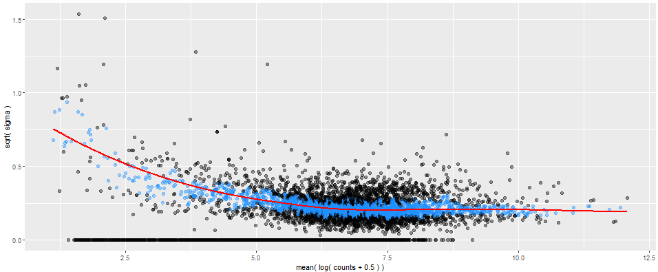
• mean-variance plot
• scatter plots
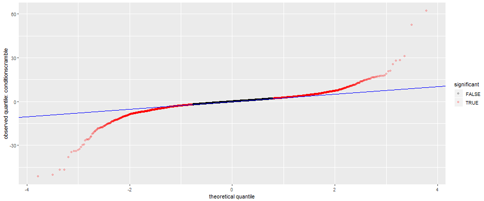
• Q-Q plot

These graphs can be used in completing a quality check and ensuring that your reads have been properly filtered.

Mean-variance plot

Q-Q plot

Understanding the data

To analyses your data, plots are available under the tab ‘analysis’